Backpropagation

What?

It’s a a part of the Gradient Descent algorithm. It’s the part in charge of actually changing the weights and biases in your neural network.

Key Idea:

Sure. As we learned in the Derivative note, you can think of the gradient of a function as the direction of the steepest slope in your high-dimensional space. But if it’s more than 3, we measly humans just can’t conceptualise that slope.

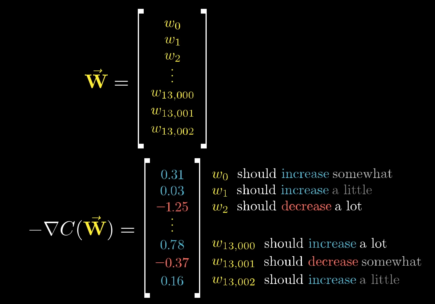
So what’s a better way of conceptualising it? Take the gradient vector, $-\nabla C(\overrightarrow{\mathbf{W}})$. Remember, each row corresponds to a weight in that layer:

• The sign of the row corresponds to whether it should increase or decrease.
• The magnitude of each corresponds to how much it should change by.

The Process, Conceptually:

1. Remember, this is just a subroutine of the larger Gradient Descent process.
2. Once we calculate the gradient of the loss function $\nabla L$, we effectively have:
   • A vector ($-\nabla C(\overrightarrow{\mathbf{W}})$) whose components tell us how much each weight should change.
3. We then update each weight:
   • Multiply each weight’s gradient by the learning rate $\eta$, which is an arbitrary constant in Neural Networks.
   • Subtract this value from the weight. (This ensures we step in the direction that reduces loss.)
   • Remember, the gradient is naturally larger if the loss is larger. So when multiplying the it by the amount to step, we make it proportional to the slope. Thus, we take big steps when far away from the minimum, but small steps when close. (This is good!)
4. Now, we move backwards through the network.
   • We know that each neuron in the output layer contributed to the error.
   • We adjust the weights leading into the output layer based on how much each neuron’s activation influenced that error.
5. Once we have these weight updates for the hidden layer → output layer, we propagate the error backward into the hidden layers.
   • If a neuron in a hidden layer needs to be less active, we modify the weights leading into it accordingly.
   • This “backward propagation of errors” is why it’s called Backpropagation.
6. Repeat this process for every training example in your dataset.
7. Important: In practice, you don’t update weights after every single example.
   • Instead, you batch your data, calculate the loss for that batch, compute the gradient for that batch, and then update the weights.
   • (This is the difference between Stochastic Gradient Descent and Mini-Batch Gradient Descent.)

Actually Doing That, Mathematically:

The weight update follows the same rule as in Gradient Descent:
$w_{\text{new}}=w_{\text{old}}-\eta \frac{\partial L}{\partial w}$
Where:

• $w$ represents the model parameters (weights).
• $\eta$ is the learning rate, which controls the step size in weight updates. (i.e. an arbitrary constant)
• ${\nabla }_{w}L(w)$ is the gradient of the loss function $L(w)$ with respect to $w$.

More specifically:

1. Gradient of the loss function with respect to weights:
   $\frac{\partial L}{\partial w_i}=(\hat{y}-y)x_i$
   Where $x_i$ is the actual feature.
2. Gradient of the loss function with respect to bias:
   $\frac{\partial L}{\partial b}=(\hat{y}-y)$

This means:

• If the predicted output $\hat{y}$ is too high, we reduce the corresponding weight.
• If $\hat{y}$ is too low, we increase the corresponding weight.
• This ensures the network slowly learns to make better predictions over time.

Batched Backprop:

Alternatively, if you’re doing batched backprop (almost always), you’d use:
$w_i=w_i-\frac{\eta }{m}{\sum }_{\text{batch}}({\hat{y}}^{(j)}-y^{(j)})x_i^{(j)}$
Where:

• $w_i$ represents a specific weight $i$
• $\eta$ is the learning rate, which controls the step size in weight updates. (i.e. an arbitrary constant)
• $m$ is the batch size
• $({\hat{y}}^{(j)}-y^{(j)})x_i^{(j)}$ is the formula for the weight $j$‘s gradient.

The Main Difference: With batched, you sum up every gradient in the batch and then divide by the batch count. This ends up looking a lot more “stumble-y”, but trains WAY faster.

P.S: You could also keep track of your momentum, and add another constant. That way, if you’ve been progressing quickly down the hill, your change in weight will reflect that.