How to evolve from Simple Linear Regression:
Consider LR with just a single feature. The line is given by . But what if you had more features? If you were to simply add another feature (with say and representing the new feature (or its absence)), you’d be left with:
\end{align*}$$ ##### The Downside? Look carefully. If gender is 0, it will be the original line. If it's 1, then it will be an offset to the original line. This assumes that the slope will be the same for the feature's presence or absence. ###### Counter Example: Imagine building a house price predictor, with features *'Number of Bedrooms'* and *'Far from City Center'*. The slopes would be inverses. ### Solution: > $y = \beta_0 + \beta_1x_{1}^{(1)} + \beta_2x_{2}^{(2)} + \beta_3x^{(1)}x^{(2)} + \text{noise}$ In this case, $\beta_3$ encodes the difference between the 2 slopes. But guess what? This generalises to where we were to begin with... Lol. ***Note***: The $x^{(1)}x^{(2)}$ is known as interaction terms. The bits that allows that 2 different features have 2 different slopes. ### General Model for MLR: > $y = \beta_0 + \beta_1 x_{1}^{(1)} + \beta_2 x_{2}^{(2)} + \beta_3 x_{3}^{(3)} + \ldots + \text{noise}$ ***As vectors:*** $$\begin{align*} \underbrace{\left[ \begin{array}{c} y_1 \\ y_2 \\ \vdots \\ y_n \end{array} \right]}_{y} &= \left[ \sum_{j=0}^{p} \beta_j \right] \underbrace{\left[ \begin{array}{c} x_{1j} \\ x_{2j} \\ \vdots \\ x_{nj} \end{array} \right]}_{x^{(j)}} + \underbrace{\left[ \begin{array}{c} e_1 \\ e_2 \\ \vdots \\ e_n \end{array} \right]}_{e} \end{align*}Note: is the effect of on if all the other features stay fixed
SLR Vs MLR:
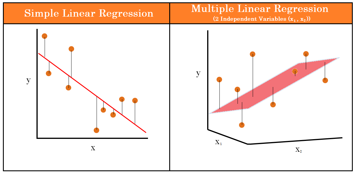
- Line + Noise Vs. Hyperplane + Noise